This example uses the default alg and enc methods (RSA-OAEP and A128CBC-HS256). It requires an RSA key.
require'jwe'key=OpenSSL::PKey::RSA.generate(2048)payload="The quick brown fox jumps over the lazy dog."encrypted=JWE.encrypt(payload,key)putsencryptedplaintext=JWE.decrypt(encrypted,key)putsplaintext#"The quick brown fox jumps over the lazy dog."
This example uses a custom enc method:
require'jwe'key=OpenSSL::PKey::RSA.generate(2048)payload="The quick brown fox jumps over the lazy dog."encrypted=JWE.encrypt(payload,key,enc: 'A192GCM')putsencryptedplaintext=JWE.decrypt(encrypted,key)putsplaintext#"The quick brown fox jumps over the lazy dog."
This example uses the ‘dir’ alg method. It requires an encryption key of the correct size for the enc method
require'jwe'key=SecureRandom.random_bytes(32)payload="The quick brown fox jumps over the lazy dog."encrypted=JWE.encrypt(payload,key,alg: 'dir')putsencryptedplaintext=JWE.decrypt(encrypted,key)putsplaintext#"The quick brown fox jumps over the lazy dog."
This example uses the DEFLATE algorithm on the plaintext to reduce the result size.
require'jwe'key=OpenSSL::PKey::RSA.generate(2048)payload="The quick brown fox jumps over the lazy dog."encrypted=JWE.encrypt(payload,key,zip: 'DEF')putsencryptedplaintext=JWE.decrypt(encrypted,key)putsplaintext#"The quick brown fox jumps over the lazy dog."
This example sets an extra plaintext custom header.
require'jwe'key=OpenSSL::PKey::RSA.generate(2048)payload="The quick brown fox jumps over the lazy dog."# In this case we add a copyright line to the headers (it can be anything you like# just remember it is plaintext).encrypted=JWE.encrypt(payload,key,copyright: 'This is my stuff! All rights reserved')putsencrypted
Available Algorithms
The RFC 7518 JSON Web Algorithms (JWA) spec defines the algorithms for encryption
and key management to be supported by a JWE implementation.
Only a subset of these algorithms is implemented in this gem. Striked elements are not available:
Permission is hereby granted, free of charge, to any person obtaining
a copy of this software and associated documentation files (the
“Software”), to deal in the Software without restriction, including
without limitation the rights to use, copy, modify, merge, publish,
distribute, sublicense, and/or sell copies of the Software, and to
permit persons to whom the Software is furnished to do so, subject to
the following conditions:
The above copyright notice and this permission notice shall be
included in all copies or substantial portions of the Software.
THE SOFTWARE IS PROVIDED “AS IS”, WITHOUT WARRANTY OF ANY KIND,
EXPRESS OR IMPLIED, INCLUDING BUT NOT LIMITED TO THE WARRANTIES OF
MERCHANTABILITY, FITNESS FOR A PARTICULAR PURPOSE AND NONINFRINGEMENT.
IN NO EVENT SHALL THE AUTHORS OR COPYRIGHT HOLDERS BE LIABLE FOR ANY
CLAIM, DAMAGES OR OTHER LIABILITY, WHETHER IN AN ACTION OF CONTRACT,
TORT OR OTHERWISE, ARISING FROM, OUT OF OR IN CONNECTION WITH THE
SOFTWARE OR THE USE OR OTHER DEALINGS IN THE SOFTWARE.
An NPM package designed for use in both browser and Node environments. It offers a range of convenient utilities specifically tailored for Arabic string manipulation, including functionalities like token search, removing diacritics and more.
Do not nest calls to ArabicString in each other it will cause undesired behavior
Example:
import{ArabicString}from"arabic-utils";// ❌ This is invalid syntaxconstnewString=ArabicString("السلام عليكم").remove(ArabicString("السَّلَامُ").removeDiacritics());console.log(newString);// ""
import{ArabicString}from"arabic-utils";// ✅ This is validconstnormalizedToken=ArabicString("السَّلَامُ").removeDiacritics();constnewString=ArabicString("السلام عليكم").remove(normalizedToken);console.log(newString);// " عليكم"
import{ArabicString,ArabicClass}from"arabic-utils";// ✅ This is also validconstnewString=ArabicString("السلام عليكم").remove(ArabicClass.removeDiacritics("السَّلَامُ"));console.log(newString);// " عليكم"
⚠️ More examples and use cases are in the test files
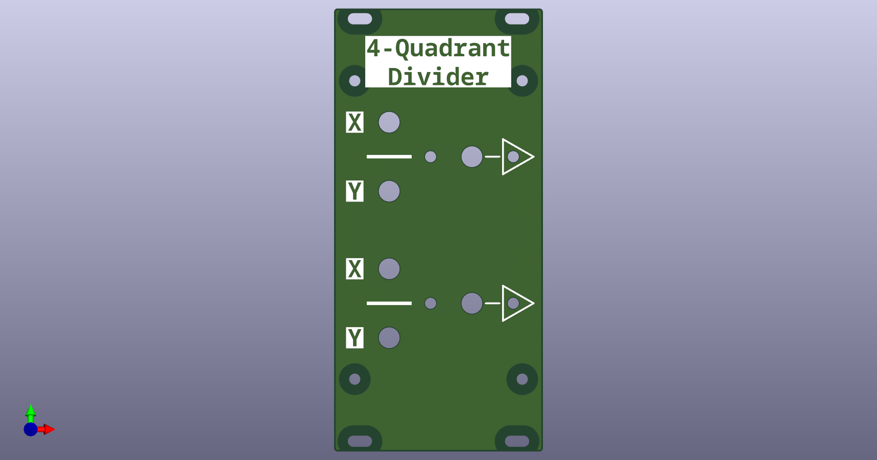
This repository provides a 4-Quadrant Division Module for analog computing applications. The design incorporates two independent 4-Quadrant Division circuits, each equipped with an output signal indicator and overload indicator to monitor operation.
The overload indicator activates if the output exceeds the machine unit of $\pm10V$ and the output signal indicator is red or green proportional to the negative or positive output voltage. This display enables easy diagnostic of an analog computing patch.
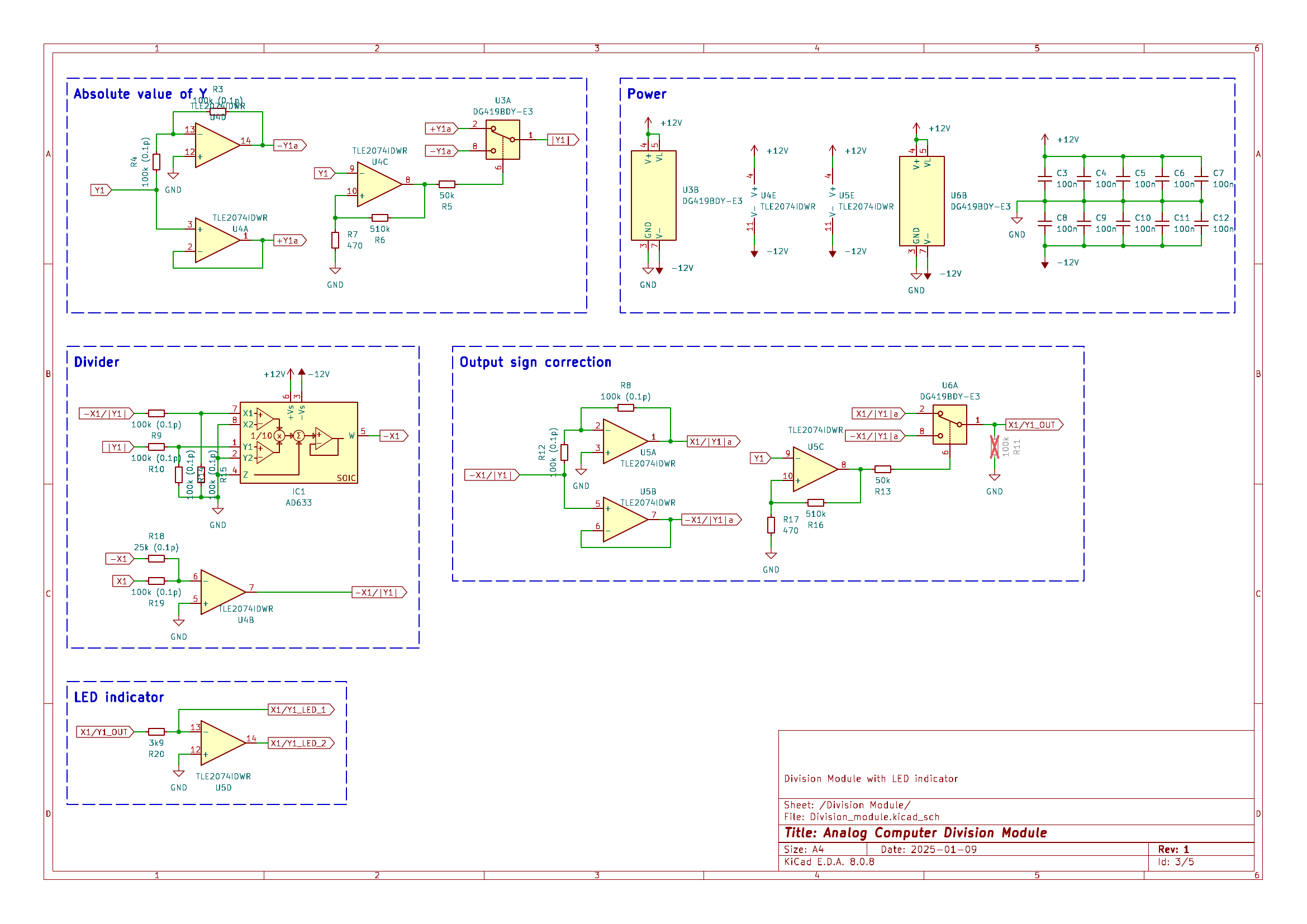
Module Schematic
The schematic is divided into multiple sections for the ease of understanding. All functional modules like power management, division and error-indication have their own page in the circuit diagram.
4-Quadrant Divider:
The division is accomplished by having the multiplier in the feedback path of an operational amplifier, thus solving for $-X/|Y|$. To cover all 4 Quadrants of the input, we first have a section to get the absolute Value of of $Y$, which is fed into the division. The output then corrects for the sign of the input $Y$ and inverts the signal when needed. Thus the Output is $X/Y$, covering all 4 Quadrants of the input. To enable easy diagnostic and debugging of an analog patch, the LED indicator displays the polarity and size of the output signal.
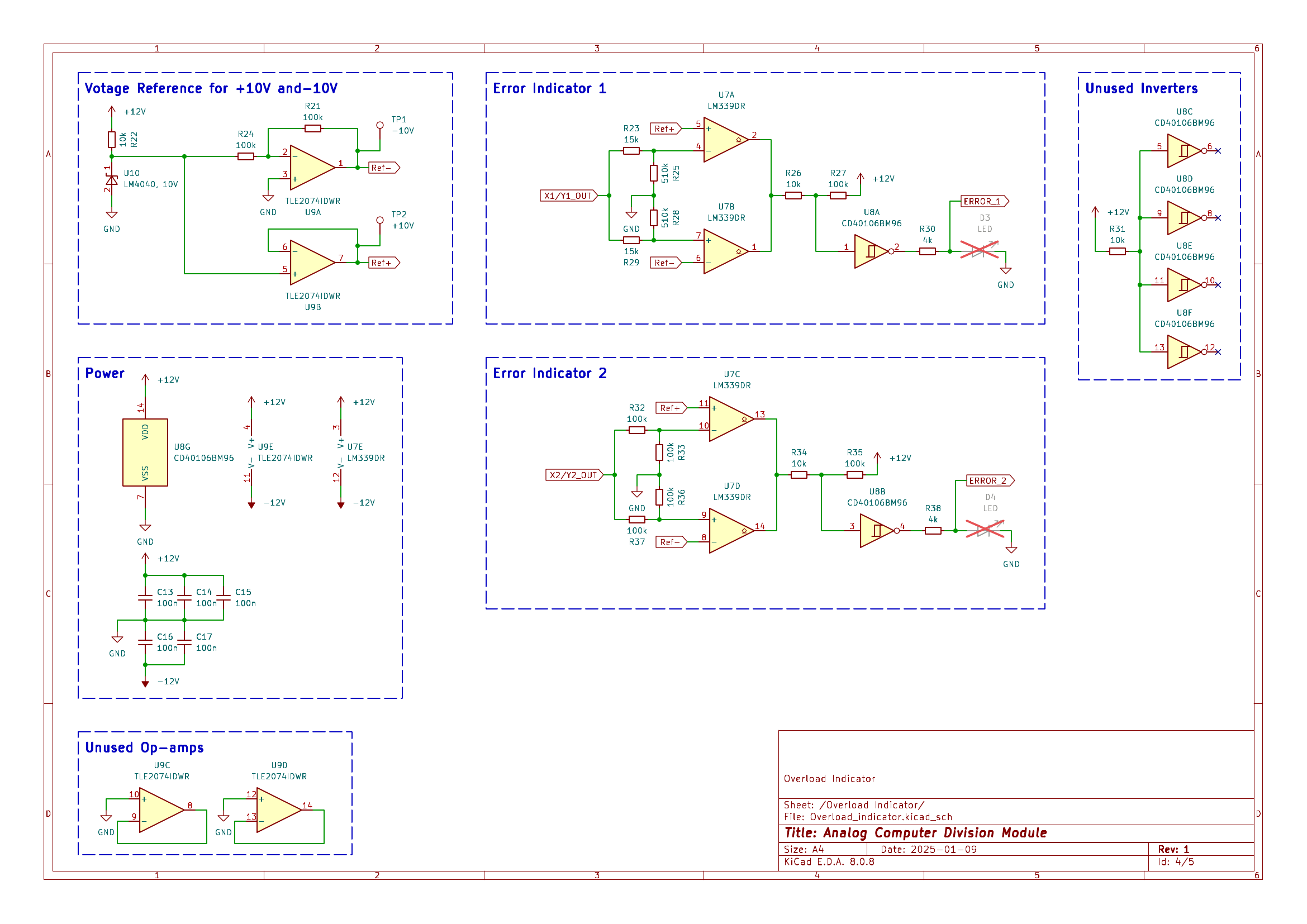
Overload Indicator:
The output signal of each seperate division circuit is compared to a reference voltage of $+10V$ and $-10V$. A red LED indicates the value of a division is exceeding the machine value of $\pm10V$. Which can easiliy happen when the absolute value of $Y$ gets small.
The Error Indicator for each individual Output takes a lot of extra space and components, but I consider it worth it for error hunting in an analog patch.
References:
The circuit is mostly based on the THAT of Anabrid GmbH, which has its circuit diagram openly available at their github repository Anabrid. Also a special mention goes to Michael Koch who has put together a large collection of analog computing circuits in his book on the THAT Analog Computer.
Set permissions on config folder so that the background service (root) can create and save the Telegram session.json:
chown root -R config
chmod 766 -R config
Optional – update path to node executable for the ExecStart property in the service file. (root’s path might differ to the logged in user / nvm’s path, and if it’s an older version of nodejs, it might break stuff…)
Create, using React, an application that should be able to calculate the appreciation/depreciation of a capital based on a monthly interest rate and time (months), using the compound interest concept.
🛠 Technologies used
CSS
HTML
Javascript
React
Hooks
Materialize
Node.js
📌Requirements
Define the elements that will be considered as application state:
capital
monthly interest rate
period
These elements will also be inputs of the application.
Inputs shall be type number
Capital value goes from 0 to 100.000, step of 100
Interest rate value goes from -12 to 12, step of 0.1
Period value goes from 1 to 36, step of 1
Output will be N boxes, being N the number of months, each one containing:
total value (amount after appreciation/depreciation of N months)
interest (value of appreciation/depreciation)
percentage (of appreciation/depreciation over the capital)
The interest rate may be positive (appreciation) or negative (depreciation).
Research and choose on of the compound interest formulas to implement.
Improve interface using Materialize.
Implementation shall use functional components and hooks.
🔍Development Tips
Use useEffect hook, with the three inputs as deps, to “watch” their change and recalculate the outputs.
TRURL 2 is a family of Large Language Models (LLMs), which are a fine-tuned version of LLaMA 2 with support for Polish 🇵🇱 language. It was created by VoiceLab and published on Hugging Face portal.
What is TRURL 2?
For most people, TRURL 2 is the least familiar term in the title above – so allow me to start here. As stated above, TRURL 2 is a fine-tuned version of LLaMA 2. According to the authors, it is trained on over 1.7B tokens (970k conversational Polish and English samples) with a large context of 4096 tokens. To be precise, TRURL 2 is not a single model but a collection of fine-tuned generative text models with 7 billion and 13 billion parameters, optimized for dialogue use cases. You can read more about it on their official blog post after the model’s release.
Even though Trurl as a word may look like a set of arbitrary letters put together, it makes sense. Trurl is one of the characters known from Stanislaw Lem’s science-fiction novel, “The Cyberiad”. According to the book’s author, Trurl is a robotic engineer 🤖, a constructor, with almost godlike abilities. In one of the stories, he creates a machine called “Elektrybałt“, which by description, resembles today’s GPT solutions. You can see that this particular name is not a coincidence.
What is LLaMA 2? 🦙
LLaMA 2 is a family of Large Language Models (LLMs) developed by Meta. This collection of pre-trained and fine-tuned models ranges from 7 billion to 70 billion parameters. As the name suggests, it is a 2nd iteration, and those models are trained on 2 trillion tokens and have double the context length of LLaMA 1.
Prerequisites and Setup
To successfully execute all steps in the given repository, you need to have the following prerequisites:
Pre-installed tools:
Most recent AWS CLI.
AWS CDK in version 2.104.0 or higher.
Python 3.10 or higher.
Node.js v21.x or higher.
Configured profile in the installed AWS CLI with credentials for your AWS IAM User account.
How to use that repository?
First, we need to configure the local environment – and here are the steps:
# Do those in the repository root after checking out.# Ideally, you should do them in a single terminal session.# Node.js v21 is not yet supported inside JSII, but it works for that example - so "shush", please.
$ export JSII_SILENCE_WARNING_UNTESTED_NODE_VERSION=true
$ make
$ source ./.env/bin/activate
$ cd ./infrastructure
$ npm install
# Or `export AWS_PROFILE=<YOUR_PROFILE_FROM_AWS_CLI>`
$ export AWS_DEFAULT_PROFILE=<YOUR_PROFILE_FROM_AWS_CLI>
$ export AWS_USERNAME=<YOUR_IAM_USERNAME>
$ cdk bootstrap
$ npm run package
$ npm run deploy-shared-infrastructure
# Answer a few AWS CDK CLI wizard questions and wait for completion.# Now, you can push code from this repository to the created AWS CodeCommit git repository remote.## Here you can find an official guide on how to configure your local `git` for AWS CodeCommit:# https://docs.aws.amazon.com/codecommit/latest/userguide/setting-up.html
$ git remote add aws <HTTPS_REPOSITORY_URL_PRESENT_IN_THE_CDK_OUTPUTS_FROM_PREVIOUS_COMMAND>
$ git push aws main
$ npm run deploy
# Again, answer a few AWS CDK CLI wizard questions and wait for completion.
Now, you can go to the newly created Amazon SageMaker Studio domain and open studio prepared for the provided username.
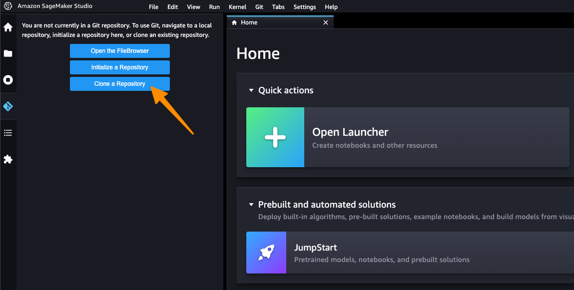
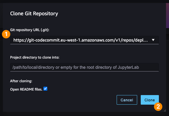
After the studio successfully starts, in the next step, you should clone the AWS CodeCommit repository via the user interface of SageMaker Studio.
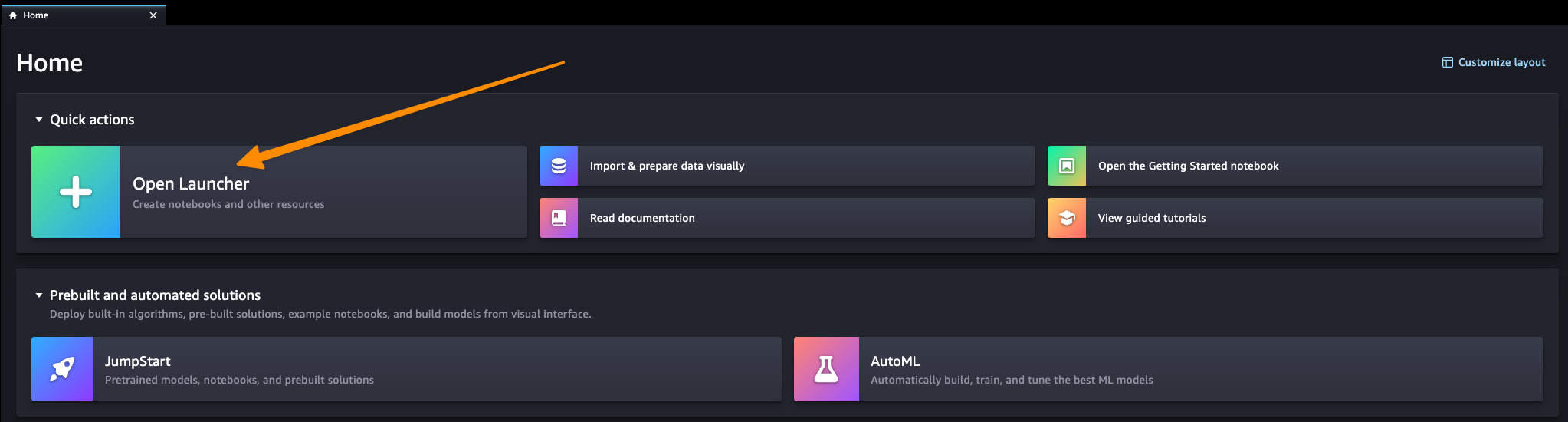
Then, we need to install all project dependencies, and it would be great to enable the Amazon CodeWhisperer extension in your SageMaker Studio domain if you would like to do that in the future on your own, here you can find the exact steps. In our case, steps up to the 4th point are automated by the provided infrastructure as code solution. You should open the Launcher tab to execute the last two steps.
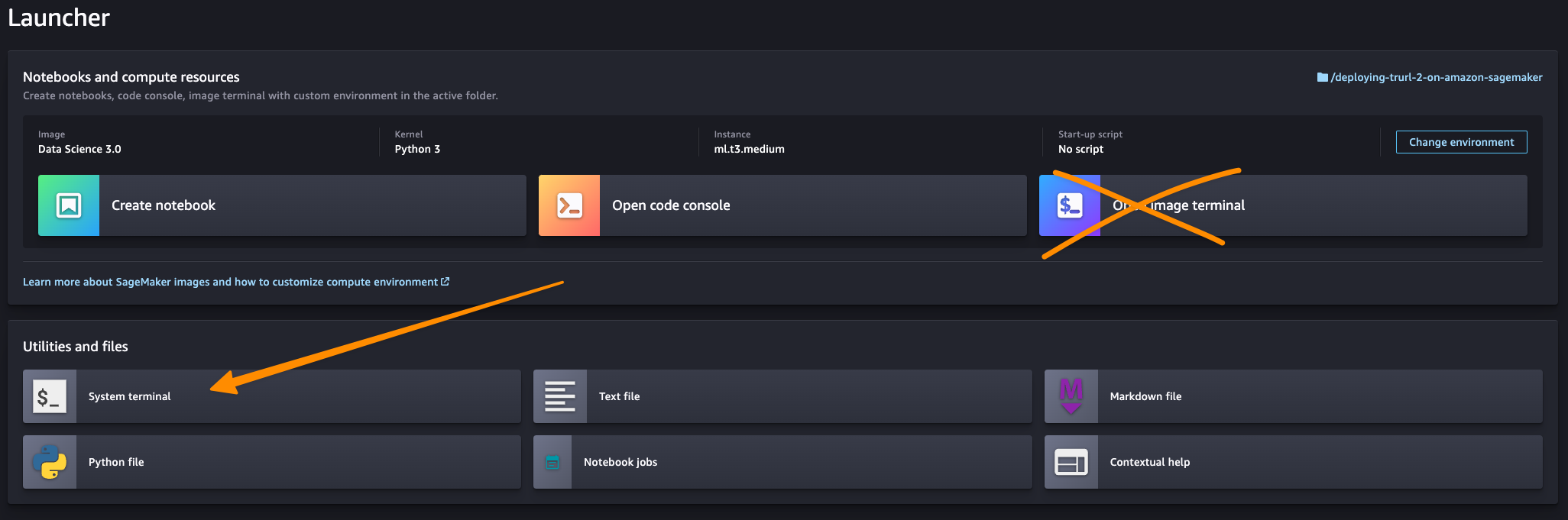
Then, in the System terminal (not the Image terminal – see the difference in the image above), run the following scripts:
# Those steps should be invoked in the *System terminal* inside *Amazon SageMaker Studio*:

$ cd deploying-trurl-2-on-amazon-sagemaker
$ ./install-amazon-code-whisperer-in-sagemaker-studio.sh
$ ./install-project-dependencies-in-sagemaker-studio.sh
Force refresh the browser tab with SageMaker Studio, and you are ready to proceed. Now it’s time to follow the steps inside the notebook available in the trurl-2 directory and explore the capabilities of the TRURL 2 model that you will deploy from the SageMaker Studio notebook as an Amazon SageMaker Endpoint, and CodeWhisperer will be our AI-powered coding companion throughout the process.
Exploration via Jupyter Lab 3.0 in Amazon SageMaker Studio
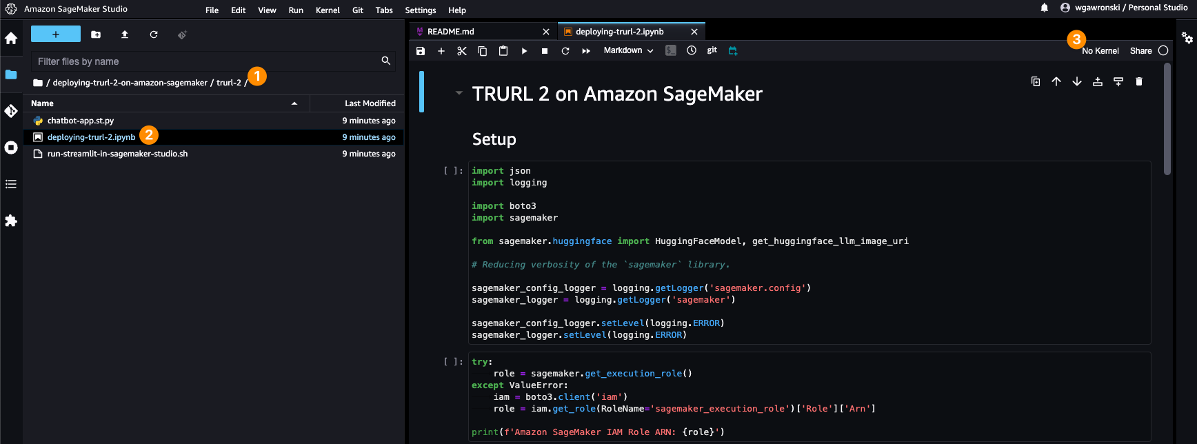
So now it’s time to deploy the model as a SageMaker Endpoint and explore the possibilities, but first – you need to locate and open the notebook.
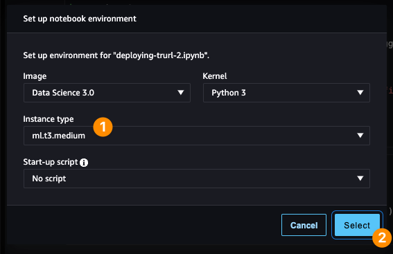
After opening it for the first time, a new dialog window will appear, asking you to configure kernel (the environment executing our code inside the notebook). Please configure it according to the screenshot below. If that window did not appear, or you’ve closed it by accident – you can always find that in the opened tab with a notebook under the 3rd icon on the screenshot above.
Now, you should be able to follow instructions inside the notebook by executing each cell with code one after another (via the toolbar or keyboard shortcut: CTRL/CMD + ENTER). Remember that before executing the clean-up section and invoking the cell with predictor.delete_endpoint(), you should stop :stop:, as we will need the running endpoint for the next section.
Developing a prototype chatbot application with Streamlit
We want to use the deployed Amazon SageMaker Endpoint with the TRURL 2 model to develop a simple chatbot application that will play in a game of 20 questions with us. You can find an example of an application developed using Streamlit that can be invoked locally (assuming you have configured AWS credentials properly for the account) or inside Amazon SageMaker Studio.
To run it locally, you need to invoke the following commands:
# If you use the previously used terminal session, you can skip this line:
$ source ./.env/bin/activate

$ cd trurl-2
$ streamlit run chatbot-app.st.py
If you would like to run that on the Amazon SageMaker Studio, you need to open System terminal as previously and start it a bit differently:
$ conda activate studio
$ cd deploying-trurl-2-on-amazon-sagemaker/trurl-2
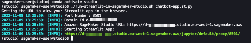
$ ./run-streamlit-in-sagemaker-studio.sh chatbot-app.st.py
Then, open the URL marked with a green color, as in the screenshot below:
Remember that in both cases, to communicate with the chatbot, you must pass the name of Amazon SageMaker Endpoint in the text field inside the left-hand sidebar. How can you find that? You can either look it up in the Amazon SageMaker Endpoints tab (keep in mind it is neither URL nor ARN – only the name) or refer to the provided endpoint_name value inside Jupyter notebook when you invoked huggingface_model.deploy(...) operation.
If you are interested in a detailed explanation of how we can run Streamlit inside Amazon SageMaker Studio, have a look at this post from the official AWS blog.
Clean-up and Costs
This one is pretty easy! Assuming that you have followed all the steps inside the notebook in the SageMaker Studio, the only thing you need to do to clean up is delete AWS CloudFormation stacks via AWS CDK (remember to close all the applications and kernels inside Amazon SageMaker Studio to be on the safe side). However, Amazon SageMaker Studio leaves a bit more resources hanging around related to the Amazon Elastic File Storage (EFS), so first, you have to delete the stack with SageMaker Studio, invoke the clean-up script, and then delete everything else:
Last but not least – here is a quick summary in terms of how much that cost. The most significant cost factor is the machines we created for and inside the Jupyter Notebook. Those are: compute for Amazon SageMaker Endpoint (1x ml.g5.2xlarge) and compute for kernel that was used by Amazon SageMaker Studio Notebook (1x ml.t3.medium). Assuming that we have set up all infrastructure in eu-west-1, the total cost of using 8 hours of cloud resources from this code sample will be lower than $15 (here you can find a detailed calculation). Everything else you created with the infrastructure as code (via AWS CDK) has a much lower cost, especially within the discussed time constraints.
This project is about an extension board for the Bluepill (based on stm32f103) I develop in my spare time.
I use this board to monitor the temperature at various places in my house, the CO2 concentration at my desktop as well as my energy consumption.
All values are polled through the network (UDP) by munin. You can even watch some live readings here.
The board is designed to be stacked on top of another expansion PCB and provides the following functionality itself:
an ethernet connection via W5500
an OneWire connector (3.3v, GND, Data)
an EEPROM socket (AT93C46W via DIP or SOIC)
temperature sensor (LM75 SOIC)
a (factory reset) button
2x status LEDs
with jumpers to disconnect them from the RTC pins (PC14 & PC15)
8x LEDs via on-board GPIO-I2C-Expander PCF8574 (SOIC)
I2C-2 connector for further frontend expansion (3.3v, GND, SDA and SCL)
(Board rev 2 connected to ethernet and with an OneWire temperature sensor)
Pinout
On the top and bottom borders the board provides the same pin-layout as the Bluepill itself.
The top row is directly connected to the Bluepill and no pin is used by the board.
Although all pins of the bottom row are used by components on the board, they are routed through nonetheless
(keep in mind that the 2×2 jumper pins can disconnect PC14 & PC15 from the board entirely – including from the bottom pins).
Gallery
Animated assembly of board rev 3.1
CO2 expansion
todo
GPIO LED Demo
todo
License
Licensed under either of Apache License, Version
2.0 or MIT license at your option.
Unless you explicitly state otherwise, any contribution intentionally submitted
for inclusion in this crate by you, as defined in the Apache-2.0 license, shall
be dual licensed as above, without any additional terms or conditions.
This project is based on the Wind-Generated-Power Prediction Hackathon by HackerEarth in 2021. The project has been made using the Pytorch library. The data which was not available were assumed to be having the values of their corresponding column. I have achieved a score of 93.5 using this model uptill now.
For preparing the data, the Pandas Library has been used extensively, since it does the job of preparing the data in the easiest manner. One hot encoding has been used to replace the text data in the dataset. The characters and their onehotencods can be found here. As mentioned earlier all the missing data has been replaced by the median values of their corresponding column.
For preparing the dataset, I have used the Dataset class imported from torch.utils.data class provided in Pytorch. Since the data is raw so, I have done the custom implementation of the same which can be found here.
Further DataLoader provided in torch.utils.data have been used while training the model.
2. Model
The model has been made by subclassing the nn.Module class provided in Pytorch. The model consists of 6 layers with 5 ReLU activation layers and 1 Softplus layer. I have trained the model for around 1500 epochs in total and to evaluate the model is not overfitting a dev set has been developed from the train dataset. The graph of loss vs iterations can also be found in above.
3. Test Set Predictions
The test set predictions can then be made and saved in a csv file.
License
Everyone is free to use it if right credits are given


 https://github.com/RubyOnWorld/jwe